Equation set

At its core, NUMO solves the incompressible Navier-Stokes momentum equation,

with a continuity equation in a form of divergence free velocity condition:

where u is the 3D velocity vector, p is the pressure and ν is the viscosity coefficient. We do not make assumptions about hydrostatic balance; therefore we use a full 3D pressure gradient term.

The forcing term G includes contributions from Coriolis and buoyancy forces. Buoyancy term is derived using Boussinesq approximation and reflects the impact of density variation on the solution:

The density variation is obtained from an equation of state, which accounts for temperature T and salinity S. Both quantities are transported using advection-diffusion equation.

Solution procedure

To solve INSE we use the classical fractional step method by Karniadakis et al. [1] with stiffly-stable time integration scheme. This projection method was shown by Guermond and Shen [2] to avoid problems with the inf-sup condition, and so is an excellent choice for high-order CG/DG discretizations. The procedure consists of three steps:

1. Evaluate the non-linear term

In the first step the non-linear and forcing terms are evaluated explicitly to find a velocity prediction ^u:where u^n is the velocity vector at time n, J_i and J_e define the order of the implicit and explicit time integration step respectively, α_q and β_q are the parameters of the stiffly-stable scheme, N is the non-linear term, G is the source term, and dt is the time step size. Typically we use J_e = J_i = 2, and the parameters of the stiffly-stable scheme can be found in [1].

2. Find pressure which projects velocity prediction to divergence-free space

We want to project ^u to a divergence-free velocity ^^u by using the pressure gradient:

To find the pressure gradient which will impose the divergence-free condition (which is equivalent to mass conservation, see Equation set above) we take the divergence of the above equation and get the following:

Solving this Poisson equation for pressure requires an appropriate high-order boundary condition, which we take after [1]:

Using the pressure boundary condition in this form is crucial for ensuring high-order properties of this fractional step formulation, including the lifting of the inf-sup condition. Since we only need the pressure gradient, not the actual value of pressure, we can freely choose the reference pressure and impose Dirichlet BCs at one point in the domain to ensure the well-posedness of this problem. Solving the Poisson equation for pressure is the most computationally expensive step of the entire solution procedure.

3. Solve for velocity

Finally, we can find the actual velocity by solving the following Helmholtz problem:
where γ is another stiffly-stable scheme parameter. The boundary conditions for the Helmholtz problem are the physical boundary conditions of the problem.

Linear solver

To solve the Poisson and Helmholtz problems outlined in Solution procedure we use GMRES solver from NUMA, along with a specialized PBNO pre-conditioner [3], which was tailor-made for the atmospheric code. We have also implemented a conjugate gradient solver and are working on an appropriate pre-conditioning technique, which would not require forming the system matrix. All implicit solves in NUMO are done using matrix-free methods.

CG/DG methods

NUMO inherits the continuous/discontinuous Galerkin (CG/DG) machinery from the atmospheric model NUMA. The details can be found in [4] and [5]. Here we only briefly present selected features of those methods.

Nodal points and basis functions

In CG/DG methods, similarly like in finite elements (FE) or finite volume (FV) methods, the domain is decomposed into elements (or volumes). What is unique in CG/DG, though, is that the solution within the element is represented by high-order basis functions. In the nodal CG/DG method used in NUMO, the solution is expanded by Lagrange polynomials based on carefully selected Legendre-Gauss-Lobatto nodal points. Those nodal points form a strongly non-uniform grid within the element, and therefore the effective resolution of the method is much higher than it would follow from the element-mesh resolution.

Integration using quadratures

In Galerkin method, the equation is multiplied by a test function and integrated over each element in the domain. The integration is numerically computed using quadrature. To save computational effort, we choose to use nodal points for evaluating quadrature, which results in some terms of the equation (i.e. mass matrix, see [4]) not to be integrated exactly. This procedure is equivalent to so-called "mass lumping" popular in FE method and is advantageous because it produces diagonal mass matrix.

CG vs. DG

The distinction between CG and DG methods comes in the conditions set upon the solution by each method. In the continuous method, we require that the solution is at least C0 continuous (i.e. no jumps in the solution across element boundaries, but the jumps are allowed in the solution derivatives), while in the DG method this condition is relaxed and we allow discontinuities across element boundaries. This approach results in a different treatment of element boundaries. Once we evaluate the solution in each element separately (by the Galerkin procedure briefly outlined in the previous paragraph), in the CG method we perform a so-called direct stiffness summation (DSS), which boils down to averaging the solution across element boundaries to enforce continuity. In DG, however, we compute a numerical flux between elements to ensure consistency of the method.

The CG condition is a more severe one (and needs additional stabilization) and requires averaging with both face and vertex neighbors, increasing communication requirements. However, by storing only the edge averaged solution it allows for reducing the degrees of freedom. The DG method is a more robust method with little to no need for additional stabilization, but this comes at the cost of more degrees of freedom required to represent a discontinuous solution. In NUMO our goal is to use the DG method due to its robustness; however, both methods are supported by our numerical framework and can be tested in the ocean model.

Grid generation

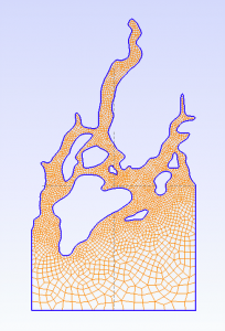NUMO has a very limited capability to generate its meshes for the flows in simple cube-like geometries. For more complicated domains we rely on Gmsh, which is a three-dimensional finite-element grid generator able to generate quadrilateral and hexahedral meshes. NUMO is capable of reading in a grid in Abaqus format, so can be used with any software.

After reading in a mesh composed of linear hexahedrons, NUMO uses the p4est library to subdivide elements to the desired resolution and distribute the mesh among parallel processes. It is important to create the smallest possible mesh that represents the details of the domain, and let p4est refine it, as this is done very efficiently in parallel. Once the element mesh is generated and partitioned, NUMO creates the nodal points within the elements.

[1] Karniadakis, G.E., Israeli, M. and Orszag, S.A., 1991. High-order splitting methods for the incompressible Navier-Stokes equations. Journal of Computational Physics, 97(2), pp.414-443.

[2] Guermond, J. and Shen, J., 2004. On the error estimates for the rotational pressure-correction projection methods. Mathematics of Computation, 73(248), pp.1719-1737.

[3] Carr III, L.E., Borges, C.F. and Giraldo, F.X., 2016. Matrix-Free Polynomial-Based Nonlinear Least Squares Optimized Preconditioning and Its Application to Discontinuous Galerkin Discretizations of the Euler Equations. Journal of Scientific Computing, 66(3), pp.917-940. [link]

[4] Giraldo, F.X. and Restelli, M., 2008. A study of spectral element and discontinuous Galerkin methods for the Navier–Stokes equations in nonhydrostatic mesoscale atmospheric modeling: Equation sets and test cases. Journal of Computational Physics, 227(8), pp.3849-3877. [link]

[5] Abdi, D.S. and Giraldo, F.X., 2016. Efficient construction of unified continuous and discontinuous Galerkin formulations for the 3D Euler equations. Journal of Computational Physics, 320, pp.46-68. [link]