A fjord model has to be able to resolve complicated geometries of Greenland, including rugged coastline and bathymetry. To achieve that, we rely on an unstructured mesh, but up until now, we have only tested the code on unstructured meshes in a box-like geometry. Even the lock-exchange test, though featuring ocean-like features, was more alike to an aquarium than a real ocean. To change that, we had to modify the way the boundary conditions are prescribed. Even though GNuMe allows for arbitrarily unstructured meshes, the atmospheric component NUMA was never required to operate on anything else than a box or a spherical shell, with boundary conditions always easily defined inside the code itself.
In the past weeks, I have implemented a feature, which allows using a mesh generator like GMSH to create an arbitrary geometry (or read it from a coastline and bathymetry database), define physical boundaries with corresponding boundary conditions, and create a quadrilateral (2D) or hexahedral (3D) mesh. The mesh, along with the boundary condition information is then read into NUMO, and the simulation is performed on this arbitrary mesh.
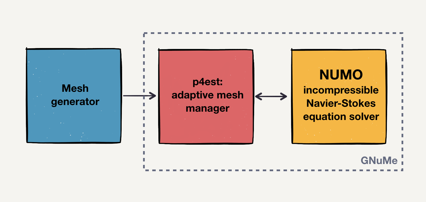
Mesh workflow in NUMO
The diagram above shows the workflow of the NUMO code. At the top level, it is composed of three stages: a mesh generator, p4est – the adaptive mesh manager, and finally the actual equation solver. The last two pieces are part of the GNuMe framework, while the choice of the mesh generator is up to the user (p4est is an independent library, but a version of it is incorporated into GNuMe).
The mesh generator creates an initial grid on given geometry and defines physical boundary conditions. This mesh can be fully unstructured with some initial (conforming) refinement, but more control over the mesh resolution is provided by p4est, and even NUMO itself. The objective of this mesh is to represent the geometry and bathymetry accurately.
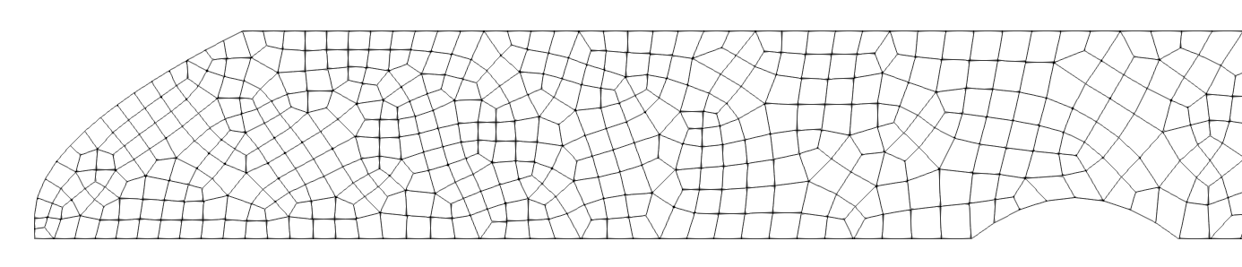
Close-up of the mesh at the “ice-cavity” (left). The bump at the bottom imitates the sill bathymetry. The domain extends further to the right (not shown).
The 2D mesh above was created for a “simplified fjord” geometry, featuring a curved ice-shelf on the left and a fjord sill at the bottom. Dimensions are not representative of an actual fjord; we have used similar length scales as in the lock-exchange case.
This grid is passed to p4est. We call it a tree mesh, or level-0 mesh, as each of the elements is a root for an adaptive octree. p4est can recursively refine each of the level-0 elements (trees). Each tree does not have to be refined uniformly, so it is not a block-structured approach, but rather a tree-refinement, which allows for non-conforming, highly-localized adaptive mesh refinement (AMR). p4est can dynamically adjust the mesh as the simulation progresses, but at this time in NUMO we only focus on a static mesh. At present, GNuMe has a capability to use AMR technology only with discontinuous Galerkin discretization, but continuous Galerkin (currently used by NUMO) implementation of non-conforming grids is under way and should be available by late 2017.
A crucial development to make a simulation like that possible was the capability of NUMO to read in the annotated boundary elements from the mesh file. This is handled by the p4est – NUMO interface, which interprets the boundary labels annotated in GMSH, and translates them to appropriate boundary condition types for pressure, velocity, temperature, etc. In the mesh above we set a no-slip condition to the ocean floor and free-slip conditions to all other surfaces. Even though the ice-shelf surface is a solid wall and would physically require a no-slip condition, we used a free-slip to check how this condition will behave in a non-orthogonal setting.
When the mesh is received from p4est by NUMO, the code creates the polynomial expansion in each element. This provides a third layer of control over the resolution (and accuracy), as the expansion order (and thus the number of nodal points in the element) can be arbitrarily chosen at runtime. Finally, NUMO solves the incompressible Navier-Stokes equations on this multi-layer grid. In GNuMe this component can be replaced by compressible Navier-Stokes solver (NUMA), or shallow water equations (for 2D meshes only).
To illustrate the arbitrary geometry and unstructured mesh capability, I have initialized the “simplified fjord” mesh with the initial condition from the lock-exchange test. This is not, of course, representative of the true fjord scale, but gives a good indication of the behavior of the code in a non-box geometry.
Even though there is no reference to compare against, this simulation demonstrates that NUMO can use arbitrary mesh and geometry.
A careful observer will see, that towards the end of the simulation there are some plumes rising from the ocean floor. This is because a Dirichlet condition was set for the temperature field (by accident) and the temperature of the ocean floor the left part of the domain is kept at +0.5C above the reference. The bug causing this unnecessary boundary conditions was already fixed, and updated simulation results are on the way.