Another checkpoint on the road towards realistic fjord simulations was a three-dimensional simulation with inlet – outlet boundary conditions in a fjord-scale geometry. I chose the density current on a slope, since this case was previously tested both experimentally (e.g. Monaghan et al. 1999) and numerically (Özgökmen et al. 2004). The goal of this idealized set-up is to mimic the bottom gravity currents that provide dense water from marginal seas to general circulation. In the case of a fjord, the dense water will flow from general circulation into the fjord, so this test checks a number of boxes on our validation list: features 3d non-hydrostatic flow, uses anisotropic viscosity and salinity diffusivity, and tests time-dependent boundary conditions for velocity and salinity.
The domain spans 10km by 2km horizontally, with the bottom sloping from 400m depth at the inflow, to 1km at the outflow. We prescribe no-slip boundary condition at the ocean bottom, free-slip conditions at the ocean surface and domain sides. Salty water (dS=1psu) is placed at the top of the slope. The salinity initial condition is perturbed in the y direction such that a fully three-dimensional flow is eventually triggered. At the inlet, we prescribe a velocity profile which satisfies the boundary conditions and has a zero net mass flux, such that the salty water near the bottom comes in, and the fresh water near the surface gets out of the domain. The magnitude of incoming velocity is adjusted to match 80% of the transient front speed, so starts at 0m/s and quickly ramps up to a relatively constant value. A salinity profile matching the initial salinity distribution is also prescribed (for details see Özgökmen et al. 2004). At the outflow, we prescribe a no-stress condition, which allows the fluid to escape the domain.
This test is also an opportunity to validate a recent development of anisotropic viscosity, which is a common feature of ocean simulations due to vastly different horizontal and vertical scales. Following Özgökmen et al. 2004, we have chosen the values of horizontal and vertical viscosity to be 


Mesh for this case is designed in GMSH, such that elements sizes vary from 50m near the bottom to 200m at the ocean surface. I have initially created an unstructured vertical mesh (in x-z plane) and then extruded it horizontally along y axis such that element size along y is also 200m. This was my initial 3D mesh, which was passed to NUMO. NUMO, using p4est, refined the mesh by one level, subdividing each element into eight smaller ones. I chose 4th order polynomial expansion in each element, which brought the effective resolution to approximately 6.25m near the bottom and 25m near the surface in the x-z plane, with 25m resolution in the y (perpendicular) direction.
Above is the visualization of the salinity field. The contours represent S>0.1psu, with warmer colors indicating saltier water. The unstructured x-z plane initial mesh is shown in the background (the actual mesh is refined by one level, i.e. each 2d element is subdivided into four smaller ones, plus there are nodal points within each element, depending on the expansion polynomial order). The front reaches the outflow in under 10000s. To compare the results with literature, we plot the evolution of front speed 
^{1/3}")


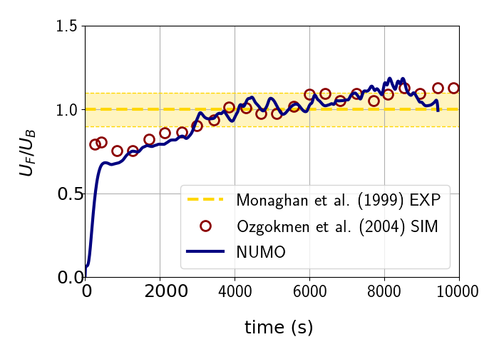
We see that the results are in a very good agreement with both simulation (circles) and experiment (dashed line with a yellow band for error range). Towards the end of the simulation, the measurement of front position is affected by the front reaching the outflow. The front seems to decelerate, while in fact some of it already traveled through the domain boundary and the measurement of average position is affected. The initial front acceleration seems to be slower in our case than in Özgökmen et al. 2004, which can be attributed to slightly different inflow condition set-up. In the middle part of the simulation, where the front has a relatively steady velocity, the match between our simulations is excellent. This result brings us a step closer to realistic fjord simulations, as it validates NUMO’s prediction of 3D buoyancy driven flows in realistic geometry scales.
As an aside, I wanted to make a quick comparison between two simulations of seemingly the same resolution, to illustrate the impact of the polynomial order on the simulation results. I used the initial mesh generated in GMSH, but rather than subdividing the elements in p4est, I have doubled the polynomial order. With 8th order polynomials, we get effectively the same average distance between nodal points but compare the animation below to the previous one. You will notice that 8th order simulation has more detail and structure, indicating a better-resolved flow. Even though we use roughly the same number of points, higher order polynomials carry more information per point and thus provide better accuracy.
So this begs the question – is it fair to compare simulations based on resolution only? Not when you are comparing different numerical methods, apparently. So what would be a better metric? Obviously, a time to solution is a solid choice – but it also involves an overall performance of the code, the kind of machine the simulation was run on, etc. What is your take on this?
References:
Monaghan, J.J., Cas, R.A.F., Kos, A.M. and Hallworth, M., 1999. Gravity currents descending a ramp in a stratified tank. Journal of Fluid Mechanics, 379, pp.39-69.
Özgökmen, T.M., Fischer, P.F., Duan, J. and Iliescu, T., 2004. Three-dimensional turbulent bottom density currents from a high-order nonhydrostatic spectral element model. Journal of Physical Oceanography, 34(9), pp.2006-2026.